2.13 Series Conditioning

2.13 Series Conditioning

The Series Conditioning functions are used to corrector condition the source data so that it displays correctly in downstream functions.

2.13.1 STEPPED

The Stepped function forces the interpolation algorithm to hold the previous value until a new value is seen. This is essential in the following cases:

• Sparse data that applies for periods of time, for example forecasts; there may be one value per month and it applies for the whole month.

• Binary or discrete data that has not been flagged as stepped in the underlying source*. For example 0 or 1 values, motor running/stopped signals etc. The motor cannot have a state between running and stopped.

* This is a parameters supported by industry standard data historians that identifies a tag as discreet (Boolean, Digital, on/off etc.)

Tip

If tag is configured as stepped in the source, this calc will do nothing and is not necessary.

The syntax for a STEPPED function is:

STEPPED(a)

a — any valid timeseries source — see section 2.2

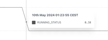
Example

The example below shows that without using the STEPPED function the RUNNING_STATUS shows an implausible value of 0.38 when trended because the underlying tag is not properly configured in the source.

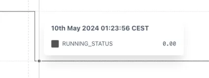
This can be fixed by wrapping the tag in a STEPPED function. Now the change in state properly shown.

2.13.2 STEPPEDRAW: Stepped Raw

The STEPPEDRAW function is identical to the STEPPED function other than it forces the use of Raw data, even if the Trend is set to Interpolated mode.

This is especially useful for reports where one needs to return an accurate total.

Use case

Forcing a TOTALISE calculation to correctly sum a forecast over a month. If the forecast has the following data:

Month	Rate	Monthly Vol.
01-Jan 00:00	1 m3/d	31 m3
01-Feb 00:00	0 m3/d	0 m3

If the Forecast rate is totalised for January without forcing the data to be stepped, then the totalizer will interpolate between 1 and 0 over January and the result will be:

TOTALISE(Rate, MONTH, BEGIN_MONTH, 1d) = 15.5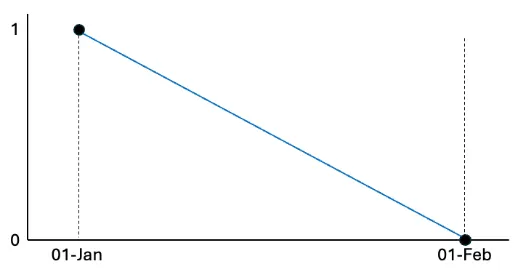

If the Rate is wrapped in a STEPPEDRAW tag it will force the calculation to step the underlying data and the result will be correct.

TOTALISE(STEPPEDRAW(Rate), MONTH, BEGIN_MONTH, 1d) = 31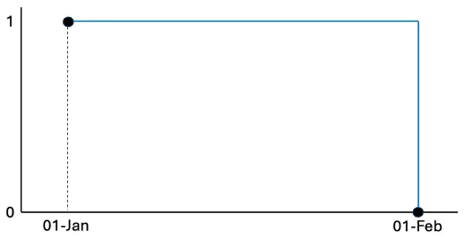

2.13.3 NOBAD: No BAD

The No Bad function removes points from the timeseries that have a “Bad” quality according to the OPC standard[^2] (possible options are Good, Uncertain or Bad) in Raw mode only.

The syntax for a NOBAD function is:

NOBAD(a)

a — any valid timeseries source — see section 2.2

This function has very limited use cases but can help if a tag has randomly incorrect data (i.e. both positive and negative) that cannot be otherwise filtered out.

Because it depends on the raw data, it’s performance can be slower than other functions.

2.13.4 TIMESHIFT

The TIMESHIFT calculation is used when the source data has an incorrect timestamp. This could be because of an incorrectly set timezone or the recording device may have the wrong time. The syntax for a TIMESHIFT function is:

TIMESHIFT(a, offset)

a — any valid timeseries source — see section 2.2

offset — an expression describing how far to shift the data back in time — see below for options

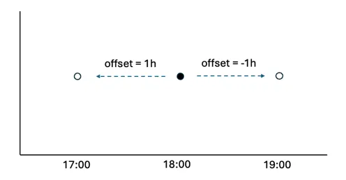
The offset is the amount of time that the source data is away from the time that you want it to be. For example, if a data point is recorded as 06:00 but it should be 07:00 then the data is “1h behind”, so the offset is “-1h” or “-01:00”.

The offset is added to the time range of the data requested so that, if a chart shows data between 12:00 - 14:00 and the TIMESHIFT function has an offset of “1h”, it will return data from the source between 13:00 — 15:00. This has the effect of moving values to the left on a trend. i.e.

Positive values shift data to an earlier point in time.

The offset can be defined in several ways. Positive values shift data to an earlier point in time:

• number of milliseconds (3600000 = 1 hour)

• an exact time definition (1s, 1h, 7d etc.) — see section 2.2 Values can be both positive and negative.

• A time expression in hh:mm or hh:mm:ss. For example, to correct a value that is 2minutes and 14 secs slow you would use -00:02:14

•  java-style durations and periods, e.g. P1D for calendar day, PT24H for exactly 24 hours

• relative time expressions, like “2 hours ago” — see section 2.4.

Examples

Retrieve value of tag at end of previous day:

"calc/TIMESHIFT(calc/TOTALISE2(constants/1, MONTH, BEGIN_MONTH,
1d), **last moment of yesterday**)",

Retrieve value of tag at end of previous day relative to another date

calc/TIMESHIFT(calc/TOTALISE2(constants/1, MONTH, BEGIN_MONTH, 1d), last
moment of yesterday)"

2.13.5 HIGHPASS

The HIGHPASS function applies a filter to a timeseries that lets the high frequencies pass and filters out the low frequencies. The syntax for the HIGHPASS function is:

HIGHPASS(tag, cutoff)

tag - any valid timeseries source - see section 2.2

cutoff - a value in second that defines the cutoff frequency. E.g. 3600 will allow peaks that occur up to an hour apart

Note that

HIGHPASS= tag – LOWPASS(tag, cutoff)

And vice-versa

2.13.6 LOWPASS

The LOWPASS function applies a filter to a timeseries that lets the high frequencies pass and filters out the low frequencies. The syntax for the LOWPASS function is:

LOWPASS(tag, cutoff)

tag - any valid timeseries source – see section 2.2

cutoff - a value in seconds that defines the cutoff frequency. E.g. 3600 filter out peaks that occur less that an hour apart